In Part 1 we worked out why FlashAttention is fast, the memory wall, and the streaming-softmax trick that lets us read Q, K and V from HBM exactly once.
In this post we will see how to turn that algorithm into an actual Triton kernel running on a GPU. We’ll write the forward pass, add causal masking, convince ourselves it’s correct, then fuse Rotary Positional Embeddings (RoPE) directly into the kernel, including the bugs and the Triton-version wall I hit along the way. Finally we benchmark it against PyTorch.
The Triton programming model
Triton lets you write a GPU kernel in Python. You don’t think about individual threads; you think about programs, where each program processes one tile of the output. You launch a grid of programs, and each one figures out which tile it owns from its program id.
For attention, the natural unit of work is one block of query rows, for one (batch, head). So the grid is two-dimensional:
grid = (N // BLOCK_Q, B * H)Inside the kernel, a program reads its coordinates and computes a base offset into the right (batch, head) slice:
block_row = tl.program_id(0) # which block of query rows
batch_head_idx = tl.program_id(1) # which (batch, head)
offset = batch_head_idx * stride_q_h
The tiles from Part 1 become block pointers, a view that says “starting from this address, with this shape and these strides, hand me a (BLOCK_Q, BLOCK_D) chunk”:
q_block_ptr = tl.make_block_ptr(
    base=Q + offset,
    shape=(N, BLOCK_D),
    strides=(stride_q_n, stride_q_d),
    offsets=(block_row * BLOCK_Q, 0),
    block_shape=(BLOCK_Q, BLOCK_D),
    order=(1, 0),
)
q = tl.load(q_block_ptr, boundary_check=(0, 1))
This is the concrete form of “load a tile from HBM into SRAM”. With , , the first program (block_row=0) loads query rows 0–3; the second (block_row=1) loads rows 4–7.
The forward kernel
The query block is loaded once. Then we stream over the K and V blocks, and inside that loop we run exactly the recurrence from Part 1. Here’s the heart of it:
for start_kv in range(0, N, BLOCK_KV):
    k = tl.load(k_block_ptr, boundary_check=(0, 1))   # (BLOCK_D, BLOCK_KV), transposed
    v = tl.load(v_block_ptr, boundary_check=(0, 1))   # (BLOCK_KV, BLOCK_D)

    qk = tl.dot(q, k) * qk_scale                      # S = Q @ K.T / sqrt(d)  (one tile)

    # causal mask
    qk = tl.where(q_idx[:, None] >= k_idx[None, :], qk, float("-inf"))

    # --- streaming softmax (Part 1) ---
    new_mi = tl.maximum(mi, tl.max(qk, axis=1))       # m_new = max(m_old, m_local)
    alpha = tl.math.exp2(mi - new_mi)                 # correction factor
    p = tl.math.exp2(qk - new_mi[:, None])            # unnormalised probs

    o_acc = o_acc * alpha[:, None] + tl.dot(p, v)     # O_new = O_old * alpha + P @ V
    mi = new_mi
    li = li * alpha + tl.sum(p, axis=1)               # d_new = d_old * alpha + d_local

    k_block_ptr = tl.advance(k_block_ptr, (0, BLOCK_KV))
    v_block_ptr = tl.advance(v_block_ptr, (BLOCK_KV, 0))

o_acc = o_acc / li[:, None]                            # the single final division
Line for line, this is Part 1: mi is , li is , o_acc is , and alpha is the correction factor that rescales the running state whenever a new maximum appears. The only thing we never do is materialise the full score matrix, each qk tile lives in SRAM and is discarded after it updates the three running variables.
One subtlety: K is loaded transposed (block shape (BLOCK_D, BLOCK_KV)), so that tl.dot(q, k) directly computes without a separate transpose.
Three details that make it real
The algorithm was explained in Part 1. Turning it into a kernel surfaces three details worth calling out, because each one is a small window into how the hardware actually works.
1. Why exp2 instead of exp
You may have noticed tl.math.exp2 instead of exp, and a scale that looks odd:
qk_scale = scale * 1.44269504089 # scale * log2(e)
...
p = tl.math.exp2(qk - new_mi[:, None])
GPUs have a fast hardware instruction for , but not for . So instead of computing , we compute , which is identically equal, we just pre-fold the factor into the scale. Its the same math, but cheaper instruction.
2. Causal masking, and a free optimisation
A causal model can’t attend to the future, so a query at position may only see keys at positions . We enforce it by setting the disallowed scores to before the softmax:
qk = tl.where(q_idx[:, None] >= k_idx[None, :], qk, float("-inf"))If a whole K block sits entirely in the future of the current query block, every one of its scores becomes and contributes nothing. So we need not even load it. Stopping the loop at the query block’s own diagonal gives, for the later query blocks, roughly half the work:
kv_end = (block_row + 1) * BLOCK_Q
for start_kv in range(0, kv_end, BLOCK_KV):
    ...
3. The 16-wide rule for tl.dot
tl.dot runs on the GPU’s tensor cores, which only multiply fixed-size tiles, the shared inner dimension must be at least 16.
Correctness before speed
It is important to test your logic against pytorch
out = flash_attention(q, k, v)
ref = F.scaled_dot_product_attention(q, k, v, is_causal=True)
torch.testing.assert_close(out, ref, atol=1e-2, rtol=0)
A tip from experience: a logic bug often hides under the high tolerance.
Fusing RoPE into the kernel
RoPE in two paragraphs
Attention is blind to word order, doesn’t know where tokens sit. RoPE fixes this not by adding a position vector, but by rotating each query and key by an angle proportional to its position. Split a vector into pairs of coordinates; pair at position is rotated by angle , where the per-pair speeds run from fast to slow.
The payoff: when a rotated query at position meets a rotated key at position , their dot product depends only on . Absolute positions cancel. And RoPE only ever touches and — never — and only affects the scores. So in the kernel it sits in right before tl.dot(q, k), and nothing downstream changes.
Where it goes
There are two honest ways to add RoPE:
- Rotate outside the kernel. Apply RoPE to and in plain PyTorch, then feed the rotated tensors into the unchanged attention kernel.
- Fuse it. Rotate inside the kernel, in SRAM, so you never write rotated / back to HBM.
Fusing trades a little redundant compute for saved memory traffic. Because each query block streams over all K blocks, a fused kernel re-rotates each K block once per query block, its redundant work, but it avoids a full round-trip of rotated / through HBM. Whether that’s a win is an empirical question, which is exactly what the benchmark below address.
First Bug
My first fused version indexed the cos/sin tables with the same offset used for Q/K/V:
offset = batch_head_idx * stride_q_h
cos = tl.load(Cos + offset + ...)
But the cos/sin tables have shape (N, D), they have no batch or head dimension, because the rotation for a position is the same for every batch and head. The first program looked fine; everything else read garbage. The kernel already computes q_idx and k_idx for the causal mask, those are the positions, so RoPE just reuses them.
Second Bug
The clean way to write the rotation is to split a loaded tile in half and recombine:
x1, x2 = x[:, :D//2], x[:, D//2:] # slice a loaded tile
x_rot = tl.cat([-x2, x1], axis=1) # swap halves, negate one
return x * cos + x_rot * sin
This didn’t compile: slicing a loaded tile raised unsupported tensor index. The fix that avoids both is a small algebra trick. Instead of stitching the rotated halves back into one tile, keep them apart and fold the rotation into the QK dot as two half-width matmuls, using the fact that a dot product over the full head-dim equals the sum over each half:
So we load each half with its own block pointer, rotate with plain arithmetic (no cat), and do two tl.dots and add. No tile slicing anywhere.
A worked example
Let’s assume Q, K, V to be this
tensor([[[[0.3581, 0.1616, 0.5714, 0.4795],
          [0.5468, 0.3008, 0.9154, 0.3457],
          [0.4201, 0.1406, 0.2273, 0.5269],
          [0.1441, 0.1024, 0.8580, 0.8310],
          [0.7828, 0.5347, 0.0038, 0.2535],
          [0.3112, 0.3961, 0.2596, 0.3704],
          [0.7789, 0.6267, 0.0297, 0.9068],
          [0.9708, 0.1654, 0.0144, 0.4128]],

         [[0.7147, 0.2785, 0.6463, 0.7070],
          [0.0046, 0.2647, 0.3889, 0.6876],
          [0.3702, 0.3406, 0.5874, 0.0967],
          [0.2227, 0.3751, 0.3261, 0.0857],
          [0.1634, 0.6659, 0.6811, 0.6651],
          [0.7258, 0.4927, 0.7543, 0.2057],
          [0.1071, 0.8613, 0.2727, 0.3571],
          [0.1453, 0.2662, 0.1778, 0.9726]]],


        [[[0.6436, 0.7744, 0.0494, 0.0897],
          [0.8326, 0.0759, 0.1208, 0.3943],
          [0.5721, 0.9949, 0.4025, 0.8175],
          [0.3231, 0.4774, 0.9158, 0.3784],
          [0.9886, 0.4412, 0.2792, 0.2915],
          [0.7545, 0.5258, 0.3754, 0.5061],
          [0.1726, 0.5226, 0.8953, 0.3112],
          [0.2522, 0.9481, 0.3493, 0.3176]],

         [[0.9558, 0.9222, 0.7712, 0.1684],
          [0.7397, 0.6067, 0.9695, 0.3222],
          [0.6258, 0.9842, 0.9909, 0.3784],
          [0.1019, 0.5079, 0.9599, 0.1936],
          [0.7737, 0.6805, 0.4499, 0.2204],
          [0.2879, 0.6809, 0.8073, 0.9478],
          [0.4164, 0.1058, 0.6489, 0.4592],
          [0.4539, 0.3612, 0.0810, 0.8282]]]])
Let’s trace block 0 with the same toy setup as Part 1 (, so ), taking for the first head. Block 0 loads positions 0–3, split into halves:
q1 (cols 0-1)        q2 (cols 2-3)
[0.3581, 0.1616]     [0.5714, 0.4795]
[0.5468, 0.3008]     [0.9154, 0.3457]
[0.4201, 0.1406]     [0.2273, 0.5269]
[0.1441, 0.1024]     [0.8580, 0.8310]
The per-pair speeds are , so position has angles . We load the first half of the cos/sin tables for positions 0–3 (the two halves of the table are identical, so the first half is enough):
cos                       sin
[ 1.0000,  1.0000]        [0.0000, 0.0000]   ← pos 0: no turn
[ 0.5403,  0.9999]        [0.8415, 0.0100]   ← pos 1
[-0.4161,  0.9998]        [0.9093, 0.0200]   ← pos 2
[-0.9900,  0.9996]        [0.1411, 0.0300]   ← pos 3
Rotate with two lines, q_rot1 = q1·cos − q2·sin and q_rot2 = q2·cos + q1·sin:
q_rot1                    q_rot2
[ 0.3581,  0.1616]        [ 0.5714,  0.4795]   ← pos 0 unchanged (cos=1, sin=0)
[-0.4748,  0.2973]        [ 0.9547,  0.3487]
[-0.3815,  0.1300]        [ 0.2874,  0.5296]
[-0.2637,  0.0774]        [-0.8291,  0.8337]
Position 0 comes out identical to the input, no turn, and the further down the block, the more the values swing. That’s the position being stamped in. Now the scores, as two half matmuls summed:
qk = q_rot1 @ k_rot1ᵀ + q_rot2 @ k_rot2ᵀ
[ 0.7108  0.5907  0.3026 -0.1559]
[ 0.5907  1.3469  0.6789 -0.3526]
[ 0.3026  0.6789  0.5255  0.3139]
[-0.1559 -0.3526  0.3139  1.4580]
which is the same for what you’d get by rotating the full vectors and doing one dot, this is just the distributive law. From here the causal mask and the streaming softmax from Part 1 take over unchanged, and is never touched.
A more detailed walkthrough of this example is in the comments, feel free to go through it
Benchmarks
All numbers are forward-pass only, causal, fp16 (with fp32 accumulation), on a mostly idle RTX 4090, , , . Timing uses triton.testing.do_bench (25 warmup iters, 100 measured,
L2 flushed between reps), reporting the median. FLOPs are counted as for the two matmuls, halved for causality, so “achieved TFLOP/s” is comparable across implementations.
Baselines: a naive PyTorch implementation (materialises the full score matrix) and torch.scaled_dot_product_attention, which in fp16 dispatches to the FlashAttention-2 backend.
fp16 matters here sine SDPA only uses its FA2 backend in fp16/bf16.
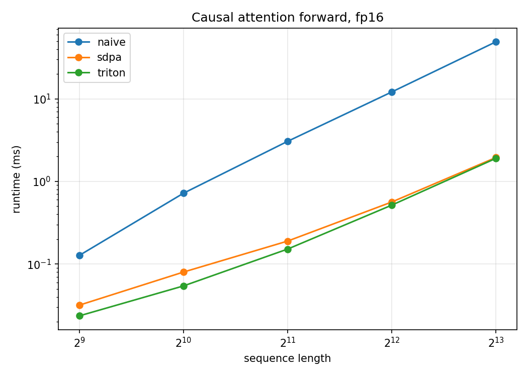
Runtime (ms) vs sequence length
| seq_len | naive | sdpa (FA2) | ours (triton) |
|---|---|---|---|
| 512 | 0.127 | 0.032 | 0.024 |
| 1024 | 0.719 | 0.080 | 0.054 |
| 2048 | 3.056 | 0.189 | 0.152 |
| 4096 | 12.104 | 0.563 | 0.516 |
| 8192 | 48.970 | 1.946 | 1.902 |
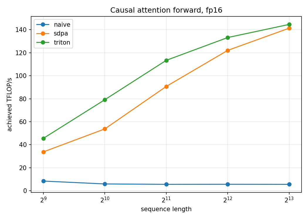
Achieved TFLOP/s vs sequence length
| seq_len | naive | sdpa (FA2) | ours (triton) |
|---|---|---|---|
| 512 | 8.5 | 33.8 | 45.6 |
| 1024 | 6.0 | 53.8 | 79.1 |
| 2048 | 5.6 | 90.7 | 113.4 |
| 4096 | 5.7 | 122.0 | 133.2 |
| 8192 | 5.6 | 141.3 | 144.6 |
Interpreting The Results
The kernel matches FlashAttention-2 across the whole range and is meaningfully ahead in the mid regime, 113 vs 91 TFLOP/s at , 133 vs 122 at and stays a little ahead at the longest sequence (147 vs 141 at ). I want to note something here: I have not beat pytorch FA2. It’s that in this specific regime, forward pass only, fp16, on a single RTX 4090, a hand-written Triton kernel reaches the same throughput as PyTorch’s FA2 backend, and edges ahead at mid lengths most likely because FA2 carries dispatch overhead and is tuned for the harder training/backward case.
Putting that ~145 TFLOP/s in context: the RTX 4090’s fp16 tensor-core ceiling with fp32 accumulation is roughly 165 TFLOP/s, so the kernel is running at about 88% of peak at long sequences. The naive baseline is flat near 5–8 TFLOP/s regardless of length, because it’s bandwidth-bound: it writes and re-reads the full score matrix from HBM, exactly the memory trap Part 1 discussed about. It’s also the only implementation whose memory grows quadratically.
One optimisation: the causal early-stop
The single change that really showed improvement was the causal early-stop discussed earlier, only looping over K blocks up to the query block’s own diagonal. It’s worth quantifying,. Here is the kernel’s achieved TFLOP/s with and without it, same config:
| seq_len | without early-stop | with early-stop |
|---|---|---|
| 512 | 45.6 | 45.6 |
| 1024 | 63.6 | 79.1 |
| 2048 | 74.9 | 113.4 |
| 4096 | 78.3 | 133.2 |
| 8192 | 78.8 | 144.6 |
Without it the kernel plateaus around 78 TFLOP/s; with it, throughput nearly doubles at long sequences (79 -> 145 at ). The reason being causal means half the work: without the early-stop, every query block still computes scores for the future K blocks and then masks them to , roughly half the matmul work, thrown away. The effect is negligible at (the first query blocks have little future to skip) and grows with sequence length, which is precisely the shape of the gap above.
Does fusing RoPE actually help?
Three ways to get RoPE + causal attention, fp16, same config:
| seq_len | rotate-outside + SDPA | rotate-outside + our kernel | fused (our kernel) |
|---|---|---|---|
| 512 | 0.073 | 0.071 | 0.028 |
| 1024 | 0.137 | 0.126 | 0.062 |
| 2048 | 0.285 | 0.260 | 0.179 |
| 4096 | 0.770 | 0.731 | 0.623 |
| 8192 | 2.554 | 2.486 | 2.344 |
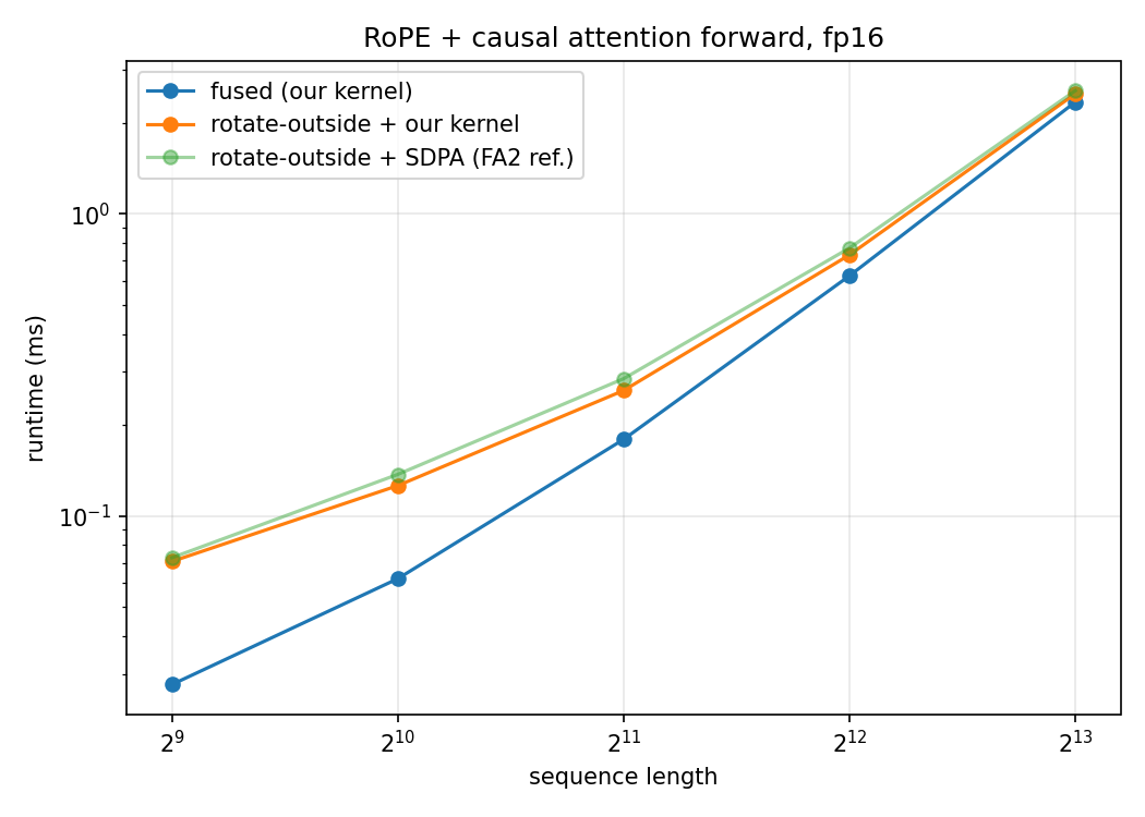
My first run had the fused kernel using a block while the base kernel used , and it showed fusion losing at long sequences, at the fused kernel took 3.19 ms versus 2.49 ms for rotating outside. That looked like fusion stops paying off past some length. Setting both kernels to reversed the conclusion: fused now wins at every length, from 2.5x at down to 1.06x at . The earlier long-sequence loss was mostly the tiles under utilizing the tensor cores, not the fusion.
So the finding is that fusing RoPE is a consistent win, with a margin that shrinks as sequences grow (2.5x -> 1.06x). That shrinking margin is the tradeoff we discussed. Fusing saves the launch overhead The savings dominate throughout the low and mid range, but the growing rotation cost gets to them, which is why the speedup decays toward 1. Extrapolating, the lines might cross at some much larger .
A note on the columns: rotate-outside + SDPA changes two things relative to the fused kernel, where RoPE happens and the attention engine (FA2 vs ours). The clean comparison is the middle column, rotate-outside + our kernel, which holds the attention engine fixed and varies only where the rotation happens.
The first version looked completely fine. fusion stops paying off past 2K. I’d have believed it. The only reason I didn’t is that the two kernels happened to differ in a second way, and that made me to recheck. The fix took one line and reversed the conclusion.
What’s next
The forward pass now sits at ~88% of peak, so the next step is the backward pass, which is where most of the real difficulty (and most of the FLOPs) actually live. Beyond that: an ncu profile to
confirm why the RoPE fusion margin decays with sequence length, the redundant K-rotation might be the suspect, and extending RoPE to long-context.
The code for everything here is on GitHub. If you spot a bug in the kernel, do let me know.